Interpolation & Splines (scipy.interpolate)
Interpolation constructs a smooth function that passes exactly through known data points to estimate unmeasured values in between.
1. Beware Runge’s Phenomenon
Fitting a single high-degree polynomial through equispaced points creates violent oscillations near the boundaries (Runge’s phenomenon). In modern engineering:
- Never fit high-order global polynomials to equispaced points.
- Use piecewise cubic polynomials (splines) instead.
# A plotting script for generating the Runge phenomenon figure
import numpy as np
import matplotlib.pyplot as plt
from scipy.interpolate import BarycentricInterpolator

f = lambda x: 1.0 / (1.0 + 25.0 * x**2)
x_nodes = np.linspace(-1, 1, 11)
poly = BarycentricInterpolator(x_nodes, f(x_nodes))
x_dense = np.linspace(-1, 1, 500)

plt.figure(figsize=(8, 4))
plt.plot(x_dense, f(x_dense), 'k-', label='True f(x)')
plt.plot(x_dense, poly(x_dense), 'r--', label='Degree 10 Polynomial')
plt.plot(x_nodes, f(x_nodes), 'bo', label='Sample Nodes')
plt.ylim(-0.5, 1.5)
plt.title("Runge's Phenomenon: Boundary Oscillations")
plt.legend()
plt.tight_layout()
plt.savefig('public/modules/scipy/ch06_runge.png', dpi=300)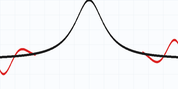
Figure 6.1: High-degree polynomial oscillation near boundaries compared to true curve.
2. Cubic Splines (CubicSpline) vs Monotone (PchipInterpolator)
CubicSpline (C2 Continuous)
Provides continuous 1st and 2nd derivatives. Default boundary condition is 'not-a-knot', which guarantees fourth-order accuracy on smooth functions:
from scipy.interpolate import CubicSpline
cs = CubicSpline(x, y)Comparing Spline Overshoot on Stepped Data
Example
Output:
3. Calculus on Splines: Fast Derivatives & Integrals
Because splines are piecewise polynomials, their derivatives and integrals can be computed analytically using .derivative() or .integrate():
Example
Output:
4. Try It Yourself
Problem: 1D Linear vs Spline Interpolation
Given sensor time series t = [0, 2, 4, 6] and readings v = [10, 14, 19, 25], estimate the value at t = 3.0 using both interp1d(kind='linear') and CubicSpline.
Show solution
import numpy as np
from scipy.interpolate import interp1d, CubicSpline

t = np.array([0.0, 2.0, 4.0, 6.0])
v = np.array([10.0, 14.0, 19.0, 25.0])

f_lin = interp1d(t, v, kind='linear')
f_spline = CubicSpline(t, v)

print(f"Linear value at t=3: {f_lin(3.0):.2f}")
print(f"Spline value at t=3: {f_spline(3.0):.2f}")