Signal Processing & Spectral Analysis (scipy.signal & scipy.fft)

Sensor streams, mechanical vibrations, electrical telemetry, and acoustic signals are time-series waveforms. SciPy provides fast Fourier transforms and digital filter design routines.

1. Fast Fourier Transform (scipy.fft)

The Discrete Fourier Transform (DFT) decomposes a signal into constituent sinusoids. For real-valued time series, always use scipy.fft.rfft (Real FFT), which omits redundant negative frequencies.

Amplitude Recovery & Frequency Bins

For a tone $A \cos(2\pi f_0 t)$, the true peak amplitude is recovered via: $\text{Amplitude} = \frac{2 \cdot |X[k_0]|}{N}$

2. Spectral Leakage & Window Functions

When a tone does not fit an integer number of cycles within the sample record, energy leaks into neighboring frequency bins (spectral leakage). Multiplying by a window function (Hann, Hamming, Flat-Top) forces the signal smoothly to zero at both ends:

# A plotting script for generating the windowing comparison figure
import numpy as np
import matplotlib.pyplot as plt
from scipy import fft
from scipy.signal import get_window
 
fs, N = 1000.0, 1000
t = np.arange(N) / fs
# 50.5 Hz tone (non-integer cycles over 1 second)
x = 3.0 * np.cos(2 * np.pi * 50.5 * t)
 
plt.figure(figsize=(8, 4))
for w_name, col in [('boxcar', 'k--'), ('hann', 'b-'), ('flattop', 'r-')]:
    w = get_window(w_name, N)
    X = fft.rfft(x * w)
    amp = 2.0 * np.abs(X) / w.sum()
    freqs = fft.rfftfreq(N, 1 / fs)
    plt.plot(freqs[:150], 20 * np.log10(amp[:150] + 1e-12), col, label=w_name)
 
plt.ylim(-80, 15)
plt.title("Spectral Leakage: Boxcar vs Hann vs Flat-Top")
plt.xlabel("Frequency (Hz)")
plt.ylabel("Magnitude (dB)")
plt.legend()
plt.tight_layout()
plt.savefig('public/modules/scipy/ch07_windowing.png', dpi=300)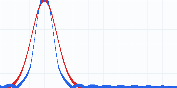

Figure 7.1: Windowing attenuates sidelobe leakage at the expense of mainlobe width.

3. Power Spectral Density via Welch’s Method (welch)

A single raw periodogram of noise has 100% relative error that does not diminish by taking longer records. Welch’s method averages overlapping windowed periodograms, reducing variance:

4. Digital Filter Design: Always Use output='sos'

When designing IIR digital filters (Butterworth, Chebyshev, Elliptic), high-order filters parameterized by transfer-function polynomials b, a suffer catastrophic polynomial-root sensitivity.

Designing and Verifying a Butterworth Low-Pass Filter

5. Peak Finding on Sensor Streams (find_peaks)

scipy.signal.find_peaks identifies local maxima. Use prominence rather than absolute height to prevent drifting baselines from corrupting detection:

6. Try It Yourself

Problem: Clean a Signal with Zero-Phase Filtering

Design a 2nd-order Butterworth low-pass filter with cutoff $40\text{ Hz}$ at $f_s = 500\text{ Hz}$ in 'sos' format. Test its frequency response gain at $10\text{ Hz}$ and $150\text{ Hz}$.

import numpy as np
from scipy import signal
 
fs = 500.0
sos = signal.butter(2, 40.0, btype='low', fs=fs, output='sos')
_, h = signal.sosfreqz(sos, worN=[10.0, 150.0], fs=fs)
gains = 20 * np.log10(np.abs(h))
 
print(f"Gain at 10 Hz : {gains[0]:.2f} dB")
print(f"Gain at 150 Hz: {gains[1]:.2f} dB")