Verification Toolkit & Engineering Capstones

In professional engineering, a number output by code is a claim. A claim demands evidence before it can be trusted.

1. The 8-Method Verification Checklist

Before accepting numerical simulation results into a design or report:

2. Capstone 1: Dynamic System Identification

A test rig with mass, spring, and damper is excited by a step force $F = 10\text{ N}$. A displacement sensor records motion at $100\text{ Hz}$ for $8\text{ seconds}$ with noise $\sigma = 1.5\text{ mm}$. We identify:

• Static gain $G = 1/k$
• Natural frequency $\omega_n$
• Damping ratio $\zeta$

# A plotting script for generating the system identification figure
import numpy as np
import matplotlib.pyplot as plt
 
np.random.seed(2024)
F = 10.0
t = np.linspace(0, 8, 800)
G_true, wn_true, zeta_true = 0.02, 5.0, 0.15
wd = wn_true * np.sqrt(1 - zeta_true**2)
y_true = F * G_true * (1 - np.exp(-zeta_true * wn_true * t) / np.sqrt(1 - zeta_true**2) * np.sin(wd * t + np.arccos(zeta_true)))
y_noisy = y_true + np.random.normal(0, 0.0015, size=t.size)
 
plt.figure(figsize=(8, 4))
plt.plot(t, y_noisy * 1000, '.', color='tab:gray', alpha=0.5, label='Noisy Sensor Data')
plt.plot(t, y_true * 1000, 'r-', lw=2, label='Fitted Step Response')
plt.title("System Identification: 2nd-Order Step Response Fit")
plt.xlabel("Time (s)")
plt.ylabel("Displacement (mm)")
plt.legend()
plt.tight_layout()
plt.savefig('public/modules/scipy/ch09_system_id.png', dpi=300)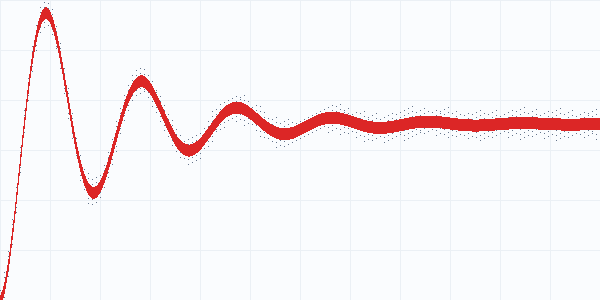

Figure 9.1: Fitted 2nd-order dynamic step response with uncertainty quantification.

Running the Parameter Extraction with Uncertainties

3. Capstone 2: Transient Cooling Process

A $40\text{ mm}$ thick steel slab ($L = 20\text{ mm}$ half-thickness) leaves a furnace at $600^\circ\text{C}$ and is cooled by air convection at $25^\circ\text{C}$ with $h = 250\text{ W}/(\text{m}^2\cdot\text{K})$. Thermal properties: $k = 45\text{ W}/(\text{m}\cdot\text{K})$, $\rho = 7800\text{ kg}/\text{m}^3$, $c = 500\text{ J}/(\text{kg}\cdot\text{K})$.

Dimensionless Biot number: $\text{Bi} = \frac{h L}{k} = \frac{250 \cdot 0.02}{45} \approx 0.1111$

Finding the Center Cooling Time

We find the time $t$ for the center of the plate to drop to $100^\circ\text{C}$ using the analytical series with brentq:

4. Try It Yourself

Problem: Verification via Residual Test

A colleague provides an empirical formula for pipe flow friction factor: $f = 0.0185$. Check the residual of the Colebrook equation at $\text{Re} = 10^5$ and relative roughness $\varepsilon / D = 10^{-4}$: $g(f) = \frac{1}{\sqrt{f}} + 2 \log_{10}\left( \frac{\varepsilon/D}{3.7} + \frac{2.51}{\text{Re}\sqrt{f}} \right)$

import numpy as np
 
f_candidate = 0.018514
Re = 1e5
rel_rough = 1e-4
 
residual = 1.0 / np.sqrt(f_candidate) + 2.0 * np.log10(rel_rough / 3.7 + 2.51 / (Re * np.sqrt(f_candidate)))
print(f"Colebrook Residual: {residual:.2e}")

Wrapping Up